
YEN/DOLLAR, TRADE DEFICITS, AND
RECENT BOOM BUST CYCLES OF USA
by
Chih Kwan Chen
(Aug. 17, 2003)
1. INTRODUCTION
Economic globalization has made trade
imbalances among economic powers of the world expand to a significant amount.
The major deficit country is The United States of America (abbreviated
as US), and the major surplus regions are Japan and other Pacific Rim Countries.
During the path of the economic globalization, that is, since 1982, US
had experienced two major boom bust cycles, the first boom topped at the
end of 1987 and the second boom peaked at the middle of 2000. A close inspection
has found that both boom bust cycles are closely related to the explosion
and the subsequent shrinkage of US trade deficits. Furthermore, evidence
indicates that the ebb and flow of US trade deficits are driven by Japanese
Yen/US Dollar exchange rates. The purpose of this article is to lay this
study out and then discuss the reasons why the new Yen/Dollar exchange
rate driven cycles emerge under the current scheme of economic globalization.
Finally a warning is given to the impending total collapse of the world
economic order if the run away trade imbalances are not corrected.
Many economic analysts and commentators,
and some elementary economics textbooks attribute the effect of merchandise
trade balances on Gross Domestic Product (GDP) simplistically as "trade
surplus adds to and trade deficit subtracts away from GDP." According to
this line of logic, more positive trade balance, either less trade deficit
or more trade surplus, should be correlated with higher growth rate of
real GDP and vise versa. Another group of opinion frequently appear on
financial media is that in an economic boom people become more affluent
and want more luxurious life style, thus import more foreign made luxury
goods; on the other hand domestically produced luxury goods will be consumed
more domestically and will be exported less. This two effects cause the
merchandise trade balance to move toward negative direction. When the economy
is in a slump, less demand for imported foreign luxury goods and more room
to export domestically made luxury goods, thus more positive the trade
balance becomes. This second line of opinion leads to the conclusion that
faster growth in GDP should coincide with more negative trade balances
and vice versa, thus in total contradiction with the first kind of simplistic
explanation. In the next section the economic data (Ref. 1) for the
pre globalization era (from 1930 to 1981) are analyzed, and the result
supports the second line of thinking, which we call the theory of "cyclical
pattern of trade balances."
In Section 3, the study of the
economic data is extended to the current globalization period with the
emphasis put on the correlation between Japanese Yen/US Dollar exchange
rate and US merchandise trade deficit. It is found that Yen/Dollar exchange
rate leads US trade deficit by two years. The running account of why major
trend changes in Yen/Dollar exchange rate have occurred and how the changes
have been translated into the trend changes in US merchandise trade deficit
is given for the whole globalization era. Section 4 is devoted to the empirical
study of the relation between economic growth and trade balance for the
globalization era. A new phenomenon called "bridge" is observed and it
is pointed out that the bridge accurately indicates the beginning and the
end of a boom, or a bubble.
Sections 5, 6, 7 and 8 are for
the theoretical explanations of the new trade pattern. Section 5 is devoted
to the discussion how GDP report compiles trade data and why the simplistic
explanation of the effect of trade balances, that is, trade surplus adds
to GDP and trade deficit subtracts away from GDP, is not correct. In section
6 and 7 the impacts of imports and exports on the economic growth are studied
respectively. Section 8 is for some other theoretical considerations, like
why Yen/Dollar exchange rate leads US trade deficit by two years, and how
the bridge phenomena are related to economic booms and stock market bubbles.
In the final section, how the current
global economic order will unravel if the problem of huge trade imbalances
is not addressed soon is discussed.
2. PRE GLOBALIZATION ERA; 1930 - 1981
To study the relation between the
trade balances and
the economic growth, we use a correlation graph. The
vertical axis of the graph represents the annual percentage
change of real (inflation adjusted) GDP, and the horizontal
axis of the graph represents the ratio of a year's merchandise
trade deficit over the current dollar GDP of that year. Fig. 1
is such a graph covering the year 1930 to 1947. For
example, the growth rate of the real GDP of 1930 is -8.6%
and the ratio of merchandise trade surplus over the GDP of
1930 is 0.88%, so an open circle with a tag "30" is plotted
at the corresponding position in Fig 1.
Open circles in Fig. 1 are for
years 1930 to 1933. Here
we see the onset of the great depression with the real GDP
shrinking year after year and most severely in 1932. As the line "A"
shows, there is an anti correlation between
the economic growth and the merchandise trade balance, just as the
theory of cyclical trade balance pattern anticipated. Years 1934 to 1938
are represented by "X" 's. The data points of 1934 to 1937 shows the effect
of the "New Deal", that is,
large government spending had boosted the economic growth. There is
no clear correlation between the economic growth and the trade balance
during those artificially boosted years. However, as the data point of
1938 shows, the boosting effect of the "New Deal" was exhausted by 1938,
US economy had fallen back into the depression, and trade surplus expanded
substantially, again as the theory of cyclical trade balance pattern predicts.
The "H" 's in Fig. 1 represent
the years of 1939 to 1943, the years of the War. The phase of the European
War started in 1939, and US plunged into the World War II in 1940. The
resulting increased production of war related material and the price control
had really pushed up the economic growth, but we can still see the anti
correlation pattern between the growth rate and the trade balance. This
anti correlation in the war years can easily be explained by replacing
the words "luxury goods" in the theory of cyclical trade balance pattern
by the words "resources to produce war material". In the time of stepped
up production of war material, along with higher economic growth rates,
US imported more raw material for the production of weapons, and thus more
negative the merchandise trade balance became. The year 1944 to 1947 are
represented by black circles in Fig. 1. The production of war material
peaked in 1943, and thus the drop of the growth rate in 1944. The World
War II ended in 1945. The economic growth plunged precipitously due to
the stoppage of production of weapons, and the trade balance turned sharply
positive due to the reduction of import of raw material needed for the
weapon production. However, US was the only major economic region not scorched
directly by the war. As the rebuilding efforts in Europe and Asia took
hold, US became the factory of the world to supply the needed material
to Europe and Asia, and this push of export had employed idled capital
and labor and had slowed down the plunge of economic growth in 1947.
From the study of Fig. 1, we only
see one positive correlation between the economic growth and the trade
balance in 1946 to 1947 which happened in a distressed situation, but witness
numerous occasions of anti correlation between the economic growth and
the trade balance; this is a clear rebuff of the simplistic explanation
that trade surplus adds to and trade deficit subtracts away from GDP; in
all the later years we will see this kind of anti correlation relation
appear repeatedly. The ratio of trade balance to GDP is limited to the
range of -0.2% to 1.2%, except two abnormal years 1946 and 1947 as
discussed before. It is the GDP growth rates that are pushed up and down
widely by various events, like the great depression, New Deal, the plunge
into the war and the ending of the war. As the economy jumps into a new
phase according to the push and pull of those events, the anti correlation
between the growth and trade balance is visible within each phase of the
economic environment as the theory of cyclical trade balance pattern predicts.
In the years covered by Fig.1 we can confidently say that drastic events
were driving the economic growth rates, and in turn the economic growth
rates were more or less determining the trade balances within each phase
as the theory of cyclical trade pattern indicates.
Fig. 2 is for the years from 1948
to 1981.
The open circles represent data for the years
from 1948 to 1966. The line labeled "A"
indicates the existence of an anti correlation
relation between the growth rate of real GDP
and the ratio of merchandise trade balance over
the total amount of GDP. There were two
exceptional years, 1954 and 1958 that are
located far away from the line "A", but rather
fit well into the next phase of line "B". The reason
of large deviation in those two recession years
and why they fit well into line "B" will not be
analyzed here. The "X" 's represent years from
1967 to 1976. The line labeled as "B" represent
the anti correlation line of this phase. This period
was plagued by the malaise of Vietnam War, and
seems that was the reason of economic phase
transition from "A" to "B". In the phase "B" there is an exceptional
year 1974, that was the year of the first oil shock. US Trade balance deteriorated
and the economy went into a recession due to the spiraling oil price. However,
after the oil shock, the economy had moved back to the phase "B". The black
circles are the years of 1977 to 1981, the time of the second oil crises
and very high inflation rate in US due to irresponsible monetary policies
of Carter administration. The line "C" is the anti correlation line of
this phase. The remarkable feature of this phase is that the data points
are so well collimated along the line "C". It is also interesting to note
that the aberration year, 1974, of phase "B" rather fits well into phase
"C".
In Fig. 2, the growth rates of
real GDP are limited to the range of +9% to -1% for all three phases. It
is rather the trade balances that distinguish those phases. The anti correlation
lines "A", "B", and "C" are persistently shifting toward the left, in the
direction of negative trade balances. Since the major factor in defining
economic phases is the trade balances, not the growth rate as in Fig. 1,
we are not sure that the anti correlation lines in Fig. 2 are the result
of the theory of cyclical trade balance pattern; it is also possible that
it is the trade balances that were determining economic growth rates rather
than the other way around as in the theory of cyclical trade balance pattern.
However, we have not found any convincing source that had driven trade
balances during the period of Fig. 2. Therefore, for convenience we still
refer the anti correlation lines of Fig. 2 as those of the theory of cyclical
trade balance pattern.
3. GLOBALIZATION, TRADE DEFICITS AND YEN/DOLLAR EXCHANGE RATES
The economic globalization under
consideration is an environment within which merchandise trade barriers
have been steadily eliminated to allow unprecedented growth in the amount
of merchandise trades. The exchange rates among the major currencies of
the world are allowed to float, though the currency markets free from government
intervention are far from reality. The economic phase marked by line "C"
in Fig. 2 can be considered as the transitional period for the world to
enter this stage of economic globalization. It is not possible to
pick one firm date and say that from that date on it is the age of globalization.
However, for the convenience of discussion we choose 1982 as the start
of economic globalization; the reason of this choice will be made clear
soon.
The marked phenomena in the process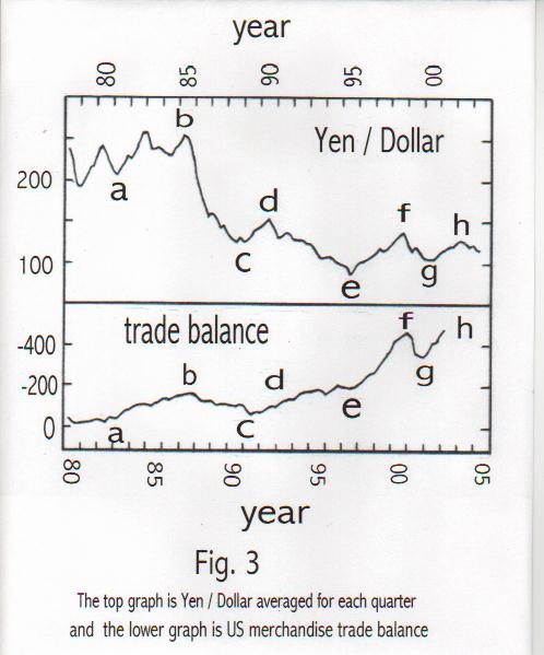
of the economic globalization are the explosive
expansions of US merchandise trade deficits
and the matching striking accumulation of
merchandise trade surpluses of Japan and other
Asia Pacific Rim Countries. A close inspection
reveals that US merchandise trade deficit is
driven by the Japanese Yen/US Dollar exchange
rates. In Fig. 3 annualized US merchandise trade
deficits are plotted for quarterly interval in the
bottom half of the graph. The minus sign in front
of the numbers along the vertical axis is to
emphasize that those numbers represent deficits.
The horizontal axis displays the years, starting at
1980. In the top half of Fig. 3 quarterly averages
of Japanese Yen/US Dollar are plotted, but with
the time scale on the horizontal axis shifted by two
years to the right. Thus the Yen/Dollar graph starts
at 1978. The major landmark points on both graphs
are marked by "a", "b", ... "h".
We will not discuss small wiggling
features of both graphs in this article, but only look at the gross characters
of both graphs. There is a remarkable matching of tops and valleys of the
two graphs except the stretch from "d" to "e"; the reason of this anomaly
will be discussed later on. This coincidence between two graphs indicates
that the ups and downs of US merchandise trade deficits are mainly driven
by Yen/Dollar exchange rates since the event in the top graph happens two
years before the corresponding events in the bottom graph. For example
the strong Dollar vs. Yen from 1981 to 1985, marked by "a" to "b" in the
top graph translated into expanding US merchandise trade deficit from 1983
to 1987, marked by "a" to "b" in the bottom graph, and so on.
Before going back to the correlation
graph as we did in Fig. 1 and Fig. 2, let us go through the events according
to the marked points in Fig. 3. First we will scan through the movements
of Yen/Dollar before the times of Fig. 3. Japanese Yen was released from
the fixed rate, 360 Yen/Dollar, at the beginning of 1970's and was allowed
to float. The market rate immediately followed the exchange rate at the
black market and US Dollar fell quickly against Yen; the Yen/Dollar rate
dropped to 265 Yen/Dollar by 1973. Then the first oil crises arrived in
1974. Japan must import almost all of its oil from outside and was especially
hard hit. Reflecting the crises and the worse situation of Japan, Yen had
fallen back to around 300 Yen/Dollar. Carter administration took office
in 1987, and started a very expansive monetary policy, inviting a substantial
inflation. That was the reason why Dollar fell, starting at 1977, from
300 Yen/Dollar to 200 Yen/Dollar by the end of 1978. Paul Vocker as the
chairman of the Federal Reserve System, used the strategy of "whatever
interest rates are necessary" approach to crash the nearly run away inflation.
As the result Dollar rose against Yen. The tail of the big Dollar fall
in Carter year due to the high inflation and the Paul Vocker recovery of
Dollar are registered in the top graph of Fig. 3 as the leftmost dip and
the subsequent rise. In 1980, due to the fall of Shaw of Iran, Dollar fell
again to the point marked "a" in the top graph of Fig. 3. Through this
rather complicated and significant falls and rises of Dollar vs. Yen, US
merchandise trade deficit displayed no significant movements. The phase
transition from "B" to "C" with worsening US trade balance actually occurred
at the time when Dollar fell big against Yen. Apparently the age of globalization
had not yet dawned.
Reagan Administration took office
in 1981. At that time the American hostages held in Iran were released.
The administration pursued "both butter and gun" policy, and made the budget
deficit explode. However, Reagan Administration had insisted to finance
the huge budget deficits through the issuance of treasury securities, not
like the previous administration to just print money to cover the deficits.
Thus the long term interest rates were pushed very high at the time when
US inflation was under control; this meant that inflation adjusted real
long term interest rates in US were sustained at a very high level for
a long time. Those conditions were the fertile ground for the appreciation
of US Dollar, and so Dollar rose against Yen as shown in the top curve
of Fig. 3 from point "a" to "b". Reagan administration also started economic
globalization by negotiating a series of tariff reducing agreements. The
strong Dollar coupled with the substantially liberalized trade environment
meant that the gate was open for Japanese goods to flood the US market,
and US merchandise trade deficit exploded, with two years of time delay
from the movement of Yen/Dollar rate, as shown in the section "a" to "b"
of the lower graph of Fig. 3.
By 1985, the explosion of US merchandise
trade deficit was unmistakable, and the currency market was ready to reverse
the trend of strong Dollar to punish the imprudent behavior of running
huge trade imbalances. Also by that time, the flood of Japanese goods had
hit very hard the heavy industrious regions of US, like the Midwest, causing
frequent uttering of the phrase "rust belt" on US media; the political
pressure on Reagan Administration to do something became unbearable. Finally
in 1985, a multinational meeting was called and two strategies were decided:
(1) To upward revaluate Yen. (2) For Japanese Government to stimulate the
domestic economy to lessen the pressure of US merchandise trade deficit.
The subsequent coordinated intervention by US and Japanese Governments
in currency market became the first stone to reverse the direction of strong
Dollar, and US Dollar started a long slide as depicted in the portion of
"b" to "c" in the top graph of Fig. 3. This sharp reversal of the Yen/Dollar
exchange rate again took two years to be translated into the trend change
of US merchandise trade deficit, and it was at the latter half of 1987
that US merchandise trade deficit finally peaked and started to decline.
Sensing this sea change in the trend of US merchandise trade deficit, US
stock market panicked in October of 1987 and thus that infamous October
disaster of 1987. The reason why stock market should have panicked as the
trend of merchandise trade deficit changed will be discussed in a later
section.
The 1987 stock market crash had
brought to the end the bubble of corporate raiders, mergers and acquisitions,
and junk bond financing. The currency market, sensing the coming period
of shrinking US merchandise trade deficit, bid up the Dollar vs. Yen as
shown in the section "c" to "d" in the upper graph of Fig. 3. This rise
of Dollar reversed the declining trend of US merchandise trade deficit
two years later as shown in the section "c" to "d" in the lower graph of
Fig. 3. During this time range in the globalization scene there occurred
a new phenomenon, that is, the emergency of Taiwan as the proxy exporter
of Japan. The sharp upward revaluation of Yen had made the manufacturing
of not so sophisticated products not cost effective in Japan, so many Japanese
manufacturers moved their factory to Taiwan to use low cost labors there
to produce those goods. Since Taiwan's currency was tagged to the US Dollar,
the cost of production of those goods was not affected by the strength
of Yen. When US trade deficit started to climb again in 1991 due to the
influence of stronger Dollar started in 1989, Taiwan was ready to play
a major role as the proxy exporter of Japan. On top of this Taiwan effect,
direct export from Japan also increased due to the strong Dollar. Those
two factors made US trade deficit rise rapidly again as shown in the portion
from "c" to "d" in the lower graph of Fig. 3.
In 1987 long promised Japanese
monetary stimulation started to have effect. In couple with the retreating
Japanese trade surplus due to the sharply higher Japanese Yen, the trend
of which started in 1985, Japanese domestic spending had started to explode.
However, either based on the erroneous simplistic thinking about trade
surplus and deficit that is already discredited in the previous section,
or bent to the domestic political pressure, Japanese Government refused
to take down trade barriers against inexpensive imports from manufactured
goods to agricultural products. As the result Japanese could only direct
abundant money into one direction, the speculation on "land"; thus the
infamous Japanese land bubble had developed. Also at that time Japanese
manufacturers had started to export equipment and industrial raw materials
to Taiwan to make it a proxy exporter of Japan. This new type of export
of Japan compensated the falling direct exports to US due to very strong
Yen, and as the result the decrease of Japanese trade surplus quickly stalled.
By 1990 this new reality became so obvious, and the currency market realized
that the sharp revaluation of Yen from 1985 was not enough to bring Japan
to correct its huge trade surplus, thus another wave to push Yen up and
US Dollar down had started and continued until 1995, shown in the section
from "d" to "e" in the top graph of Fig. 3. The strategy to use Taiwan
as the proxy exporter turned out to be an enormous success and the export
from Taiwan to US exploded. Also the flow of goods from Taiwan was resistant
to strong Yen since Taiwan's currency was fixed against US Dollar at that
time. Thus in spite of the sharp increase in the value of Yen in the stretch
of "d" to "e", US Trade deficit increase was not easy to reverse. Only
at the end of the move of Yen/Dollar in the "d" to "e" section, with the
2 year delayed effect, US trade deficit started to level off as is clear
from "d" to "e" in the bottom graph of Fig. 3. As Taiwan became more
affluent by serving as the proxy exporter of Japan, people became more
outspoken in human rights, democracy, free labor movement and environmental
control; multinational manufacturers abandoned Taiwan and migrated to other
Pacific Rim Countries in search of places with lower labor costs and the
freedom to pollute the environment. During the process of "d" to "e" it
was a tug of war between the currency market that wanted to devaluate Dollar
against Yen to correct the imbalances of trades and the multinational manufacturers
that expanded the proxy exporters to nullify the intent of the currency
market to correct lopsided trade imbalances.
By the beginning of 1995, Dollar
was dropping very rapidly against Yen, and US trade deficit had started
to level off. The currency market was as if saying, "Yen/Dollar will be
dropped to whatever level is necessary to correct the trade imbalance with
US at one side and Japan and the proxy exporters at the other side." Japanese
Government panicked at the thought that Japan's huge trade surplus would
melt away, so it started an unprecedented and risky gamble, that is, to
flood the market with Yen and thus to destroy the value of Yen deliberately.
Clinton administration was worried about the first signs of stagnating
economy as US trade deficit started to level off just before the reelection
campaign of 1996, so it explicitly endorsed the gamble of Japanese Government
under the catch phrase of "strong Dollar policy". Thus the sharp upturn
of Dollar vs. Yen as seen in the section of "e" to "f" in the Yen/Dollar
graph of Fig. 3. This currency movement of 1995 was translated into a further
rapid climb of US trade deficit as shown in the section from "e" to "f"
of the trade balance graph of Fig. 3. During this currency manipulation
which is still continuing today, the currency market knows that Japanese
Government, in principle, can issue whatever amount of Yen which is necessary
and dump on the market to push the value of Yen down, so no currency trader
will stand in the way of Japanese Government. Instead the currency market
used its ultimate weapon against the manipulator, that is, as if to say,
"All right, if you want weak Yen, we will give you weak Yen and much more
until you cry out from the pain of disaster sawed by yourself." Thus with
Japanese Government leading, and currency traders pushing, Dollar steadily
advanced against Yen, US trade deficit had exploded along with the trade
surplus of Japan, US economy sustained high growth rates accompanied by
Clinton's land slide victory in 1996, and Japanese economy turned to recession
from stagnation under the weight of run away trade surplus. Then the proxy
exporters became the first major innocent victims of this currency manipulation
in the form of Asian economic crises. The currencies of those proxy exporters
were tagged to US Dollar. As the value of Dollar moved up, so were the
currencies of those proxy exporters. Very soon those proxy exporters stopped
to function as proxy exporters, and Japan resumed to export directly to
US. Since those ex-proxy exporters were too slow to detach their currency
hookup to US Dollar, hot money flew in to take advantage of interest rate
differences between their treasuries and the US treasuries based on the
false assumption that the currencies of the ex-proxy exporters could be
tagged to Dollar for a long time. Those ex-proxy exporters experienced
consumption booms due to the influx of hot money, and ran trade deficits
just like US but against a much shallower asset base. When someone shouted,
"The Emperor has no cloth", all the hot money ran to the exit at once,
and thus triggered the Asian economic crises. The crises had boomeranged
back to Japan and turned a recession into a minor depression. The details
of this Asian economic crises is analyzed in other places so will not be
repeated here (Ref. 2 reflects the author's view that the main instigator
of the crises is the currency market manipulation of Japanese Government,
Ref. 3 is a more conventional view which assigns blame on the infrastructures
of Asia Pacific Countries other than Japan and argue somehow those infrastructures
of many countries failed simultaneously.) Even with the Asian economic
crises Japanese Government had insisted on to manipulate the currency market
to destroy the value of Yen, so currency traders helped Japanese Government
to push the value of Dollar higher and higher. By 1998 the currency crises
based on the increasingly strong Dollar had spread to non Asian currencies
pegged to the US Dollar. Both Japanese Government and US Government panicked,
and engaged a coordinated intervention to brake the trend of rising Dollar.
That was the signal that the currency market was waiting for, the signal
that the manipulator had cried out from the pain of the wound opened by
itself, so the currency market pushed Dollar off a cliff. That is the first
leg of the drop recorded in the section of "f" to "g" in Yen/Dollar graph
of Fig. 3. As the currency crises spread further, another sharp drop of
Dollar in 1999 as the second leg of drop of Yen/Dollar, shown in the section
"f" to "g" in Yen/Dollar graph of Fig. 3. This sharp reversal of the fortune
of US Dollar had been translated into, with almost a two year delay, the
reversal of the rapid increase of US trade deficit in the middle of 2000
as depicted in the portion of "f" to "g" of the trade balance graph of
Fig. 3. That trend reversal in the US trade deficit then had punctuated
the bubble of US stock market.
Japanese Government, without learning
from their disastrous currency market manipulation, started another round
of Yen destruction activity at the end of 2000, apparently taking advantage
of a political power vacuum in US due to the transition from Clinton to
Bush Administration, and is recorded in the Yen/Dollar curve of Fig. 3
as the section from "g" to "h". This push up phase ended in the spring
of 2002 due to the sharp market reaction. With almost the delay of one
and one half years, US trade deficit has risen sharply again in 2002 and
will peak out near the end of 2003 or the beginning of 2004 as can be seen
in the portion from "g" to "h" in the trade balance curve of Fig. 3.
4. CORRELATION BETWEEN ECONOMIC GROWTH AND
TRADE DEFICIT IN THE GLOBALIZATION ERA
In the previous section we have
shown that the graph of Yen/Dollar rates shifted two years toward the right
direction coincides remarkably with the graph of US merchandise trade deficits,
and have interpreted this coincidence as the evidence that US trade deficits
are driven by Yen/Dollar rates with the latter enjoying a two year lead
time. The theory of cyclical trade balance patterns, which says that the
trade balances are driven by the boom and busts of the economy, does not
apply here. If we assume that the trade deficits are driven by the economy
as the theory says, then we will be forced into a rather ridiculous conclusion
that the currency market participants are super smart and they, and only
they know what is going to happen to our economic fortune two years in
the future and adjust Yen/Dollar rate at present accordingly. We do not
accept this kind of eccentric argument, so we follow the interpretation
of Section 3 that it is today's Yen/Dollar rate that determines the US
trade deficit two year down the road. The next thing we want to know is
how the merchandise trade deficit is interacting with the economic growth.
With those understandings we will be able to say that Yen/Dollar rate drives
US merchandise trade deficit and in turn the ups and downs of merchandise
trade deficit determine booms and busts of US economy.
The correlation graph between
annualized
growth of real GDP of US and the ratio of
merchandise trade balance over current dollar
GDP, for 1982 to 1997, are presented in Fig. 4
with the data point for each year tagged by a
2 digit number, indicating the year. As we follow
the data points of "82", "83" and "84", it shows
an increasing trade deficits accompanied by
stronger growth in GDP, where the exploding
trade deficits were fueled by the strong Dollar vs.
Yen during the period of "a" to "b" in the
Yen/Dollar curve of Fig. 3. 1984, with a GDP
growth rate of 7.3%, had been the only year
since 1966 that US economic growth rate had
exceeded 6%, and apparently the growth was
over the natural growth potential of US like 4 to
5 % a year. Thus the growth rate fell back to
below 5% in 1985. However, the period of the
exploding trade deficit of 1982 to 1987 was not
over, so with the growth rate stuck near the
potential growth rate and with trade deficit
exploding, data points "85", "86" and "87" moved toward left along
a horizontal line labeled as "B" in Fig. 4. In the pre globalization era
studied in Section 2, transition from a phase represented by a slanting
line like "A" in Fig. 2 to another such an inclining line of another phase
was common, but never displayed any such horizontal multi-year line like
"B" in Fig. 4. We will call the horizontal line like "B", a "bridge". The
"bridge" of 1985 to 1987 apparently coincided with the first bubble of
corporate merger frenzy, and when the data points came to the end of the
bridge, the bubble burst. 1988 was the year that the data point retreated
to the bridgehead as US trade deficit shrank due to the reversal of the
trend of trade balance as shown in the bottom curve of Fig. 3, section
from "b" to "c". As US trade deficit retreated further and further as the
time advanced, data points of 1989, 1990, and 1991 had slide down along
the line "A", ending at slightly negative GDP growth rate of 1991. Another
push upward of US trade deficit, which started at 1992, push up the data
point of 1992 along the line "A". As the trade balance curve started to
stagnate in 1994 to 1997 (see section "d" to "e" of the trade balance curve
of Fig. 3), data points of those years are clustered together in Fig. 4.
Data points of 1991 to 2002 are
plotted
in Fig. 5, with years 1991 to 1997 and the
line "A" of Fig. 4 reproduced. The phase of
further exploding US trading deficit of the
section "e" to "f" in the trade balance curve of
Fig. 3, which was induced by the massive
currency market manipulation of Japanese
Government, produced the second "bridge",
labeled as line "D" in Fig. 5. This second bridge
was the period of the most recent bubble.
When it comes to the end of this second bridge,
the recent bubble burst. However, the down
turn of US trade deficit started in 2000 has
been rather shallow due to the China factor,
since China has become the major proxy
exporter whereas the currency of China is
pegged to US Dollar. Thus the data point
of 2001 has not been able to retrace the bridge
as in the case of 1988, but rather has formed
a new phase, labeled as line "C" in Fig. 5; we
are currently still in this most recent phase.
5. HOW IMPORTS AND EXPORTS ARE TABULATED IN GDP
Starting from this section, we
will turn our attention to theoretical backgrounds of the phenomena observed
in previous sections. In this section we will consider the way imports
and exports are handled in GDP tabulation, and show why the simplistic
explanation that trade surplus adds to and trade deficit subtracts away
from GDP is clearly in error.
Let us start by following the path
of an imported article, say a shirt. Let us assume that the price of the
imported shirt is $1 at the time when it passes through the custom. As
the shirt goes through various stages of retail channel, values are added,
and suppose it is finally sold to a consumer for $10. In the GDP report
there is a category called "final sales" or "personal consumption", and
this sale of the shirt, $10, will be added to the total amount of "final
sales". However, this tabulation is not correct, since GDP should only
calculate values produced domestically, and the first dollar of the shirt
is clearly not produced domestically; in other words GDP should have booked
$9 from the sale of the shirt, not $10 as done. That is the reason that
at the end, GDP creates an additional category called "imports" to subtract
this $1 from GDP; this "imports" is simply the total amount of imported
goods tabulated at the time when they pass the custom. The mistaken simplistic
view that imports subtract away from GDP comes from just looking at the
category of "imports" and think that more we import, more we subtract from
GDP. However, in the example of the imported shirt, if we have not imported
this shirt, we certainly will not subtract $1 from GDP due to the "imports",
but we also cannot book $10 from the sale of this shirt in the tabulation
of "final sales". Thus the net effect of not importing this shirt
is negative by $9 to GDP, not plus $1 to GDP as the simplistic explanation
trying to let us believe. After saying that it is also dangerous to think
naively that more we import, more positive GDP will become, since we must
weigh carefully the impact of the import on the domestic manufacturers;
the pros and cons of imports will be analyzed in the next section.
Now how about exports? The exports
are clearly values produced domestically and should be added to GDP. However,
in the major categories of GDP report, there is no place that is tracking
the contribution of exports. That is why there is another category called
"exports" in GDP, in which the total amount of exports as they pass through
the custom are tabulated and are added to GDP. It is also erroneous to
think that more exports means more plus to GDP, since we must weigh carefully
about what happens if the item is not exported but consumed domestically;
apparently the resources used to make exports will not be available to
make domestically consumable goods. The "imports" and the "exports" categories
in GDP are usually grouped together as "net export" though they have very
different characters in GDP tabulation as discussed above; the combination
into "net export" apparently causes further confusion and lead to the mistaken
simplistic thinking that trade surplus adds to and trade deficit subtracts
away from GDP. Usually the impacts of trades on GDP depend on the economic,
social and even psychological structures of a society and must be studied
case by case. In the following two sections we will derive some general
conditions under which imports and exports will boost or depress GDP.
From the discussion in this section it
should be clear that the simplistic explanation that trade surplus adds
to and trade deficit subtracts away from GDP is based on a misunderstanding
about how trade data are used in GDP tabulation. Another caution related
to this issue is in order. For example, on Aug. 14, 2003 US June trade
deficit is officially announced by the Commerce Department, and the trade
deficit turned out to be somewhat less than expected. Financial media immediately
reported that the estimate of the second quarter GDP growth will be adjusted
upward, thus giving an impression that positive trade balance is beneficially
to GDP and vice versa. What is happening here is that as discussed GDP
tabulation compute "final sale" and "imports" separately. The personal
spending data of June came out several weeks earlier than June trade data,
so economists has already used the actual data to compute "final sale"
of the second quarter, but the "imports" and "exports" categories for the
second quarter are only based on guess. When the real data has come out,
the guess about trade balances of the second quarter then need to be adjusted.
It does not mean that positive trade balance adds to GDP as the simplistic
explanation claims. Our study based on the actual data in previous sections
has already discredited such simplistic explanation completely.
6. IMPACTS OF MERCHANDISE IMPORTS
Our major concern here is that
strong Dollar induces explosive expansion of US trade deficit, and we want
to know how this explosive increase of trade deficit will influence the
growth of US economy. Thus we must analyze how imports and exports will
influence economic growth, not the other way around as done in the theory
of cyclical trade balance patterns. In this section we will consider the
impact of imports.
There are many varieties of imports.
Here we exclude the service imports. Service imports have vastly different
characteristics from merchandise imports. For example, the money spent
overseas by a domestic traveler is counted as service import, and the money
spent domestically by an oversea-visitor is counted as service export.
Such service exports are automatically counted in "the final sales" category
of GDP, so it does not need to be added to the "exports" category of GDP.
On the other hand, traveler based service imports do not contribute to
GDP, so it should not be added to the "net imports" category either. Other
kinds of service imports and exports, like the insurance bought from or
purchased by foreign companies, are directly added to "imports" and "exports"
categories. However, this kind of service imports and exports typically
does not have any multiplying power. For example, a service worth $1 purchased
by a foreign entity, is still only worth $1 if purchased instead by a domestic
company. Thus the effect of service trades on the economy is much less
prominent compared to the merchandise trades. Therefore, in this
article we will not consider the effects of service trades.
Within merchandise trades, the
monetary amount of imports can change either due to the change of
the quantity of imports, or due to the change of the import prices. The
quantity of imports of inelastic merchandises, like oil, does not change
very much even its price fluctuates widely. The effect on GDP due to the
change of oil price is quite obvious; if the price of oil jumps, it is
going to hurt GDP and vice versa. However, the amount of oil imports of
US (about 60 billion US Dollars a year, assuming oil price at $30 a barrel),
though is large, pales when compared to the overall merchandise trade deficit
of US, which is about 500 billion US Dollar a year. Thus in this section
we will only consider the merchandise trades excluding inelastic commodities
like oil.
To understand the effects of merchandise
imports, excluding oil, we first consider a virtual society where there
is no manufacturing activity at all as a pure example. All the economic
activities of this society is service oriented, like retail sales, financial,
real estates, insurance, health cares, and, of course, the activities to
import all the required manufactured goods from overseas. If a shirt, as
in the example given in Section 5, is imported, it literally adds nine
dollars to GDP since there is no domestic shirt making activity in this
virtual society so no worker will be laid off and no factory will close
its door due to this imported shirt.
The situation of this virtual society
can be looked at from a different angle. Suppose the central bank decides
to release more money into the society by either lowering the interest
rates or by reducing the reserve requirements of the commercial banks,
whereas the total quantities of imported goods are fixed, then due to the
rule of supply (fixed amount of goods) and demand (more money), only thing
will happen to the society is inflation. Thus the nominal GDP will increase,
but the inflation adjusted real GDP will remain exactly the same no matter
how much extra money the central bank injects into the society. In order
for the real GDP to grow, the quantities of imports must also grow. Therefore,
in this virtual society, more imports means more growth in the real GDP.
In that sense we may call this virtual society "the heaven of merchandise
imports".
If the currency of this virtual society is left to the free currency
market, it will lose value quickly and the virtual society will be forced
to have manufacturing sectors since it can not afford to continue to import
large quantities of goods. Only way that the virtual society can sustain
its pure form is for the governments of other societies to artificially
buy the currency of that virtual society to support its value, just as
Japanese Government is buying US Dollar.
In a real society, there may exist
some manufacturing sectors that are exposed to the competition of imported
goods. Let us assume that the shirt making business is within such a manufacturing
sector. When a $1 shirt, as discussed in the previous section, is imported,
a domestically manufactured shirt sold, say for $1.5 by the manufacturer,
is pushed out of the market. If the capital and labor used to manufacture
the domestic shirt cannot be redeployed to other sector, then GDP will
lose this $1.5, assuming that the domestic shirt will also generate $9
if it goes through the retail channel. If the capital and labor can be
redeployed to some other sector, GDP will most likely gain since this newly
produced value will open up a new retail channel and will generate a large
sum of its own added values that is surely more than $1.5. However, if
the imported shirt does not compete with any domestic shirt, than the imported
shirt will add $9 to GDP, just like the case in the virtual society. Thus
whether imports will be beneficial to a society or not depends on how much
new opportunities exist, and how close the society is to the virtual society
without any manufacturing base.
7. IMPACTS OF MERCHANDISE EXPORTS
Some societies are gifted by nature
in some special ways, like many Middle East Countries are abundant in oil,
and US is very favorable for mass-producing agricultural goods. For those
countries, small input will yield large outputs of those naturally favored
goods. Also it is difficult for other places to replace those naturally
bestowed goods. Here we are not going to consider the export of this kind
of natural resources, but concentrate on the general merchandises that
are highly replaceable depending on the cost of production in a specific
region. We also limit our consideration of the impact of general merchandise
export on a matured, or developed economic entity; the analysis of the
impact of exports on a less matured economy, or developing country exposes
various unique, intriguing and interesting questions, and deserve to be
studied in a separate article of its own.
Let us consider a matured economic
entity growing at its maximum potential, so that its capital and labor
are fully deployed. Suppose there is a production of a shirt, and it is
valued at $1 when it leaves the factory and is sold to a consumer for $10
after going through various stages of retail channel. Thus this shirt contributes
$10 to GDP. Now suppose by some artificial intervention (like government
action) this shirt is taken out of the domestic circulation and is exported.
GDP tabulation will add $1 to the "exports" category, but the "final sales"
account will lose $10. The net effect of exporting this shirt is thus negative
by $9 to GDP. Due to this export, the capital and labor in the retail
channel to generate $9 value if the shirt had been sold domestically is
now idled. In an ideal situation, this idled capital and labor can be redeployed
to some other sector instantaneously to reproduce the lost $9. However,
even in this ideal situation the best GDP can do is to become the same
as before the export of the shirt. In real case there is always a time
delay in recouping the lost $9 due to the export, so GDP almost always
lose. This is intuitively easy to understand since when an economic entity
is growing at its maximum potential, there is simply not possible to accelerate
its GDP further without fixing its structural problems. It also points
out the impossibility to boost GDP by artificially increasing exports in
a matured economic entity under normal conditions, in total contradiction
to the simplistic explanation. Artificially increasing exports will rather
cause GDP to shrink for a matured economic entity when it is growing near
its natural potential. This is why Japan has sunk into a prolonged recession
as its government has deliberately destroyed the value of Yen in order
to make its trade surplus explode.
Only when the matured economic
entity is already in a deep recession or in a depression and there are
plenty of idled capital and labor, then by some artificial means to deploy
those idled capital and labor for producing exportable goods will help
GDP, like the case from 1946 to 1947 in US discussed in Section 2. However,
any artificial action to increase export, even under those miserable conditions,
will usually have severe side effects and the harm to its economy will
out weigh the benefit from the increased export. If a matured economic
entity is in trouble, it is better to stimulate its domestic consumption
rather than to take artificial means, like deliberately destroy the value
of its own currency in order to increase its exports.
8. YEN/DOLLAR TIME DELAY, AND BOOM BUST AND THE BRIDGE
In Section 3 we have observed that
major trend changes in Yen/Dollar exchange rate is translated into significant
shifts in the pattern of trade deficit with a time delay approximately
two years. It may be surprising to some that the change in currency exchange
rate takes so long to influence the trade balance. To answer this question,
let us consider two countries A and B, and assume that both countries have
factories to manufacture shirts for their domestic markets respectively,
and also let us assume that at the beginning the costs of manufacturing
shirts in A and in B are similar. Suppose the currency of A suddenly move
up sharply against the currency of B so that the cost to make a shirt in
A becomes substantially higher than the cost in B. The shirt company in
B will naturally take advantage of the situation by expanding its shirt
making capacity, make more shirts, export them to A, and drive the shirt
company of A out of business. In order to do this the shirt company in
B must draw up a plan, get the financing for the plan, physically expand
the shirt manufacturing facility, make more shirts, and then export to
A. All those steps take time and thus there will be a long time delay from
the currency movement to the actual trading of a shirt between A and B.
It happens to be that this unavoidable time delay is about two years in
the real world.
In Section 4 when we studied the
"bridge" phenomena, we said that those bridges correspond to bubbles. Besides
the empirical facts that the physical timing of a bridge coincides with
the era of a bubble, there are also theoretical reasons why a bridge should
be related to a bubble. As discussed in Section 6, imports will boost the
economic growth if the capital and labor displaced by the imports can be
redeployed to other fields quickly. When imports flow in too rapidly,
the ability to redeploy labor and capital will be strained and the growth
rate of GDP will hit a ceiling, whereas the ratio of merchandise trade
deficit over current dollar GDP will expand rapidly. Thus a bridge is formed
in the correlation graph like Fig. 4 and 5. In case of the Reagan era boom
and bust, the retreat of US merchandise trade deficit, starting near the
end of 1987, was significant, so the ratio of trade deficit to GDP move
rapidly toward right, and the economy settled back to the phase where the
bridge had sprung. In the boom of Clinton era the retreat of US merchandise
trade deficit, starting at 2000, is measured since the fall of Dollar vs.
Yen in 1998 to 1999, though was sharp, but was not really drastic. Thus
the US economy has not be able to return to phase "A" of Fig. 5 but has
entered into a new phase "C" in Fig. 5, which encompass a much higher ratio
of trade deficit to GDP than the previous phase of "A" in Fig. 5.
It is interesting to observe that
if a society is near the virtual society without any manufacturing base,
the "bridge" phenomenon will not appear, since in the virtual society,
more import simply means more growth assuming that the retail sector is
very elastic. Thus the data points on a correlation graph simply move toward
the upper left direction along a slanting trend line like the line "C"
in Fig. 5 if trade deficit increases. In that sense the appearance of bridges
in both the Reagan year bubble and the Clinton year bubble means that US
is still not yet near the virtual society with most of the manufacturing
sectors extinguished.
Now about the reason why a stock
market bubble often accompanies "bridge" phenomena. When US runs a merchandise
trade deficit, US Dollar is handed over to foreigners. The foreigners may
sell the dollar to other foreigners, but the net amount of the dollar will
remain in the hands of foreigners; in recent days those dollars will be
most likely ended up in the hands of foreign governments. Since US Dollar
is not legal tender in the countries with large trade surpluses, those
foreign owned dollar must be deposited back to US. The foreign dollars
in US will not buy consumers goods, but will be invested, for example,
in US treasuries. When those foreign dollars buy US treasuries, some US
investors, most likely some institutions, must sell the treasury securities
to those foreigners. The proceeds of the sale of treasury securities received
by domestic institutions then will be invested in other fields, and stock
market will benefit directly. When the merchandise trade deficit starts
to shrink, less money comes into stock market from this rout. That is why
in a period of explosive rise of merchandise trade deficit, a stock market
bubble will appear. At the time when the trade deficit starts to shrink,
less money of this trade deficit rout will come into the stock market,
and the bubble will start to burst. This kind of stock market bubble burst
cycle had appeared in Reagan era that ended in 1987, and again in Clinton
era and the bubble burst in 2000.
9. THE FUTURE OF US ECONOMY
Through out this article, we have
repeatedly advanced the claim that strong Dollar induces large merchandise
trade deficits, and the large trade deficit in turn boosts US economy and
creates bubbles. It has always been the declining trade deficits that burst
bubbles and introduce economic down turns. Some may get an impression that
strong Dollar and the delayed explosion of merchandise trade deficit, even
it is artificially introduced by the action of Japanese Government, is
our friend, and weak Dollar induced by the currency market to discourage
the huge trade imbalance, and the subsequent shrinkage of merchandise trade
deficit is our enemy. However, it is not the case. To use merchandise trade
deficit to boost economy is like to take illicit drugs to achieve temporary
stimulus; eventually it will destroy the whole economy and will reduce
an economic superpower into a second rate economic back water. Let us see
the reason of this conclusion.
From very early in the history
of humanity the accumulation of monetary commodities, like gold and silver,
is considered to be the measure of wealth. This measure applies to individuals
and also to governments. At the time when gold is used to settle trades,
if a country, which does not produce significant amount of gold, wants
to accumulate more gold, it needs to run a trade surplus. The thinking
that the goal of the economic policy of a country is to let it accumulate
more gold, or to run the maximum possible trade surplus is called "mercantilism".
Before the great depression mercantilism was the prevailing economic wisdom
of the world. After the great depression mercantilism has given way to
modern economics. Modern economics tries to evaluate the richness of a
country not based on how much gold it owns, but on the living standard
of the people of the country. However, the living standard of the people
is not easy to quantify. In the modern times when the quantification is
touted as the ultimate goal for economics to attain the similar respectability
as natural sciences, the concept of the living standard of the people is
replaced by an objective measure like GDP and its growth. In this article
we have shown that the growth of real GDP of an economic entity, and the
trade balance is mostly anti correlated, thus trade deficit is desirable
if our only goal is to achieve high growth rates of GDP. However, GDP is
only a view from one direction of the condition of an economic entity.
If we concentrate only on GDP, we are prone to fall into a folly that is
frequently uttered on many financial media: Suppose a natural disaster
befalls on Country A and destroys a large number of houses. This loss of
property will not be reflected on GDP of A, whereas the subsequent effort
to rebuild the lost houses will be recorded as big gains for GDP. Thus
many financial commentators will say something like, "The disaster is a
human tragedy, but it is a big plus for the economy." The error that those
commentators have committed is to ignore the other equally important indicator,
the "national account balance". The "national account balance" is computed
as follows: Sum the values of all assets physically based in Country A.
Add all the claims that the government, corporations and individuals of
Country A have against foreign sources, and finally subtract all the claims
that any foreign source has against the entities of Country A. The last
two terms combined together is called the "net external asset" that can
be positive or negative. Positive net external asset adds to the national
account balance, and negative net external asset subtracts away from the
national account balance. The negative net external asset is also called
the "net external debt". The national account balance is the measure to
gauge the net worth of Country A. If the national account balance dips
down to zero or negative, it is equivalent to a familiar financial condition
of individuals called "bankruptcy". When a natural disaster hits and many
houses are destroyed, it is the national account balance get reduced and
the living standard of the people of Country A is reduced; apparently it
is a highly undesirable condition for Country A. The rapid growth of GDP
in the frenzy of rebuilding only reflects the efforts to rebuild the national
account balance back to the pre disaster level. Therefore, it is purely
against common sense and against the logic of modern economics as well
to call such natural disasters as plus to the economy of Country A.
Quite a few countries in Latin
America, Asia and other places have experienced currency crises after running
significant trade deficits for some time. Those currency crises have occurred
because those countries must settle their trades with other countries in
dominant currencies, like US Dollar. When the foreign currency reserve
of the country is exhausted, its import will plummet, causing GDP to fall
sharply as discussed previously in this article. Hot money that has entered
the country under the misjudgment of its money managers will panic and
want to escape from the country. If the currency of that country is floated,
then the currency will fall drastically to cause further panic and so on
and so on until its economy collapses and requires the aid of outside entities,
like IMF. At the time of the currency crises the national account balance
of that country is usually still in black. Then how about a country like
US whose currency is widely accepted as the settlement currency of international
trades? There is no rule that US Dollar should be accepted as an international
trade settlement currency. Foreign parties accept US Dollar as the payment
for their goods only based on the historical trust built toward the Dollar.
If their confidence wanes, US Dollar will lose its value against other
currencies in the currency market. Studying the constant tug of war and
the cat and mouse type engagement between the currency market and Japanese
Government, it is fair to say that the trust of foreign private parties
toward US Dollar has waned a long time ago due to the run away US trade
deficit. It is purely due to the enormous market manipulation to destroy
the value of Yen and to support US Dollar undertaken by Japanese Government,
foreign private parties are still accepting US Dollar as the payment for
their goods since they know that they can always sell their US Dollar to
Japanese Government for other currencies.
Now let us project what will happen
in 20 years if the current condition persists. To estimate what is going
to happen in the future for US economy, we need first to understand what
is the net external debt of US at present. US net external asset turned
to zero at 1985. By adding up all the current account deficits since 1985
we will get a reliable picture of what the net external debt is at present.
At the end of 2002 it is like 3.2 trillion dollars. The net external debt
probably will grow like 550 billion dollars in 2003. Assuming that Japanese
Government, with the help from China, will support the value of Dollar
to the level that US can run a merchandise trade deficit of about 5% of
GDP, near the line "C" in Fig. 5, for a long time to come. Also let us
assume that US current dollar GDP will grow like 4.0% a year (e.g. 1.5%
inflation and 2.5% real growth), and that US service trade surplus will grow
such that the burden of financing the external debt will cancel out with
the increasing service trade surplus. Under those conditions it is possible
to estimate that at 2023 US external debt will be 18 trillion dollars and
the current dollar GDP will be about 22 trillion dollars. Further assuming
that the total value of US based assets is similar to the current dollar
GDP, then at 2023 the national account balance of US will be 22 - 18 = 4
trillion dollars. At the end of 2003, US national account balance will
be about 10.5 - 3.75 = 6.75 trillion dollars. Thus in 20 years US national
account balance will shrink by 2.75 trillion dollars, but nominal GDP, or
the consumable sums, will jump 220%, and inflation adjusted real GDP will
grow by 164%. The merchandise trade deficit will be 1.1 trillion dollars
a year. On the other side of the ledger, we need to consider what is going
to happen to Japan. Currently Japan's current dollar GDP is about
5.0 trillion dollars, and the external asset is around 1 trillion dollars
in black. This means that the national account balance of Japan is
about 6 trillion dollars. The growth of Japan's current dollar GDP is slightly
negative; if we assume deflation is 2% and the real GDP growth is 0%, then
the current dollar GDP is shrinking 2% a year in Japan. Since Japanese
trade surplus must increase to accommodate strongly expanding US trade
deficit, the ratio of Japan's trade surplus to its GDP will increase and
the growth of real GDP will slump further as we have discussed throughout
this article. Even if we are very optimistic and only assign a 3% shrinkage
a year in the current dollar GDP of Japan, the current dollar GDP of Japan
at 2023 will be like 2.7 trillion dollars. Suppose Japan holds 50% of 18
trillion dollar of US external debt, then Japan's national account balance
will be 2.7 + 9.0 = 11.7 trillion dollars at 2023, a substantial expansion
from the present level of 6 trillion dollars.
Let us translate those numbers into plain
language. The condition at 2023 will be as follows: American net worth
will shrink substantially by 2023, but an average American citizen will
live in an estate home built with money borrowed from Japan, will
drive Japanese made luxury automobiles purchased with the money borrowed
from Japan, and will dine daily in high class restaurants and charge the
expense on credit cards which are again financed with the money borrowed
from Japan. At that time US will become a virtual society, as discussed
in Section 5, without any manufacturing base. US Federal Reserve System
will become the agent of Japan, China, Taiwan, Hong Kong, and Singapore
who collectively hold 18 trillion dollar worth of claims on US. On the
other side of the Pacific, Japan will become the richest nation on
earth according to its national account balance, but an average Japanese
will be peddling bicycles instead of driving automobiles, a Japanese family
will be clamped into a 300 square feet apartment, and an average meal of
Japanese citizen will return to a box of white rice with a red preserved
plum sitting in the middle of the box, a typical diet of Japanese during
the World War II. Japanese Government will be more occupied in managing
9.0 trillion US dollar located in US than to be bothered with running a
meager 2.7 trillion Dollar Japanese domestic economy. If we think such
a picture is too ridiculous to be true, then we must conclude that US Dollar
will suffer a catastrophic collapse, the runaway US trade deficit will
be curbed, and US economy will sink into a depression on the way to 2023.
REFERENCES
1. US economic data used in this article are published by US Commerce
Department
and US Federal Reserve System.
2. Chih Kwan Chen, "Economic Crises of Japan, Asia and Beyond", (1998).
3. G. Corsetti, P. Pesenti, and N. Roubini, "What caused the Asian currency
and financial crises?
Part 1: A macroeconomic overview" (1998).
Return to the Home Page of the Website